Model comparison

Model fitting, cross-validation and posterior predictive checks

Let’s think back to the quote by George Box mentioned earlier in the course:

“Essentially, all the models are wrong, but some are useful.” - George E.P. Box (1976)

This is particularly relevant in cognitive modeling, where no model can perfectly capture human cognition. However, some models provide more useful approximations than others.

Consider our reinforcement learning example: we might have several competing hypotheses about how people learn from rewards. Perhaps some participants use a simple learning strategy with a single learning rate, while others might use different learning rates for positive and negative outcomes. Or maybe some individuals incorporate uncertainty into their learning process. Each of these hypotheses can be formalized as a different computational model, but which one best describes our participants’ behaviour?

Model comparison provides us with systematic tools to answer this question. Rather than simply accepting the first model that seems to fit our data reasonably well, we can fit multiple models and compare which is best. In relation to Box’s quote, we want to see which model is the least wrong!

Model fitting and the Goldilocks principle

Have a look at the graph below, which shows polynomials of different orders being fitted to some data, where \(M\) represents the order of the polynomial:

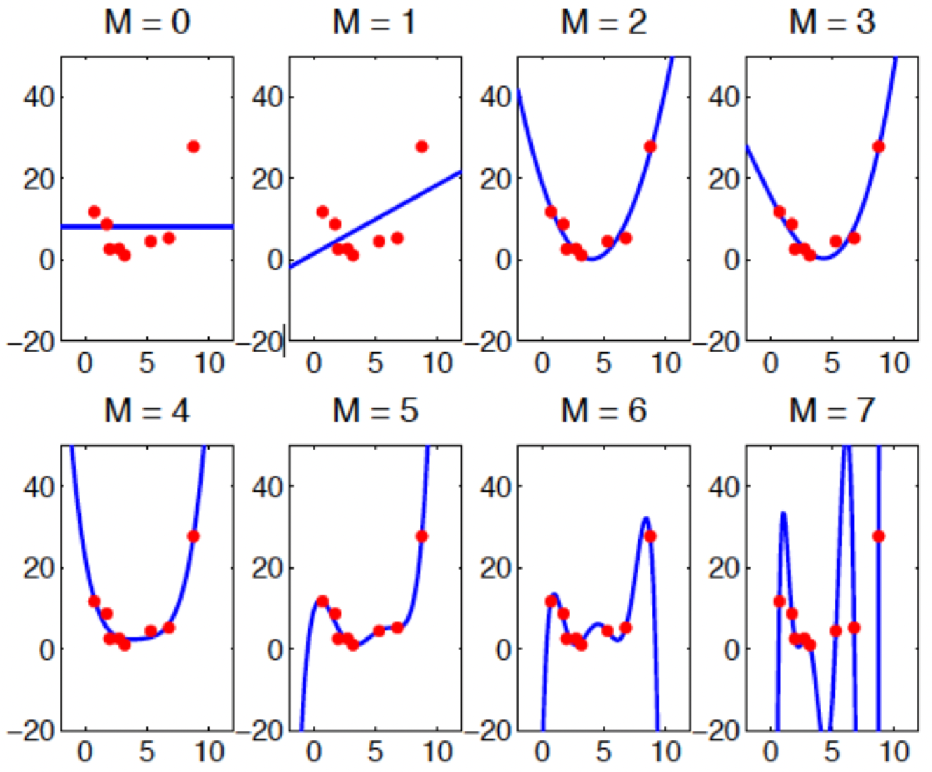
Looking at the model fits, which order-polynomial is ‘best’?

At first glance, you might think the \(M = 7\) model is ‘best’ since it passes exactly through each data point. However, this intuition leads us to the concept of overfitting - where a model learns to fit the noise in the specific data provided rather than explaining the underlying pattern more generally.

Overfitting can be humorously described by a John von Neumann quote recalled by Enrico Fermi:

“With four parameters I can fit an elephant, and with five I can make him wiggle his trunk.”

Elephants aside, his point was that with enough parameters, you can fit any pattern in your data - even if that pattern is just random noise.

This brings us to model-fitting, a fundamental concept in model selection illustrated in the figure below¹:

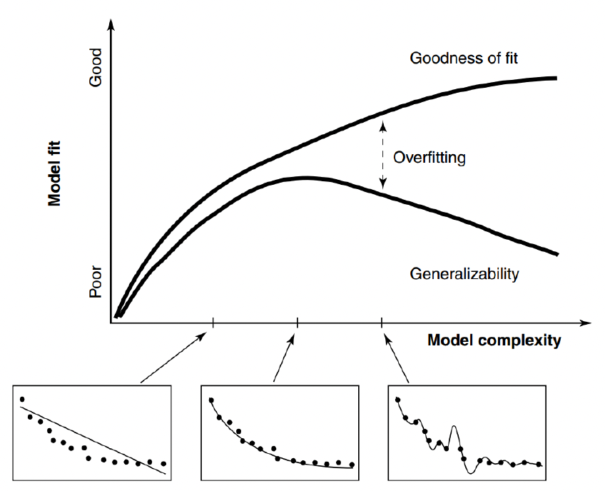
Model fitting is an example of the Goldilocks principle: it needs to be just right

The graph shows that as we increase model complexity, we initially see improvements in how well our model fits the data. However, there comes a point where adding more complexity leads to overfitting.

The figure shows two crucial curves:

The “Goodness of fit” curve shows how well the model fits the observed data, which continues to improve with complexity.
The “Generalizability” curve shows how well the model performs on new, unseen data. This curve peaks and then declines as the model becomes too complex.

Looking back at our polynomial example, while \(M = 7\) undoubedtly gives us the best fit to our observed data points, it would likely perform poorly if we tried to use it to predict new data. The model has accurately but specifically learned the noise in our sample rather than the more general relationship we’re trying to understand.

Ultimately, we need to find a sweet spot - a balance between underfitting and overfitting.

But how do we determine which model is best? A more philosophical rule follows Ockham’s razor, which (in one variation) states that:

“When having two competing theories that make exactly the same predictions, the simpler one is the better.” - original maxim attributed to William of Ockham (c. 1285 - 1347)

Specifically concerning model selection, we should therefore prefer simpler models when they provide similar explanatory power or make fewer assumptions; \(M = 2\) or \(M = 4\) might provide the best balance - capturing the main trend in the data without overfitting.

Cross-validation

As a result, we would like to know which model best fits the data but also generalizes to new unobserved data.

But how do we define and implement this objectively? One way is through cross-validation.

Cross-validation (\(k\)-fold) involves fitting a model to most of the data and testing it on the remainder \(k\) times

The basic principle is straightforward: we divide our dataset into two parts:

1. A training set that we use to fit our model

2. A validation set that we use to test how well our model predicts new, unseen data

The figure above shows a specific type: \(k\)-fold cross-validation, where the data is divided into \(k\) equal sections, and each section takes a turn being the validation set while the remaining sections form the training set.

Leave-One-Out Cross Validation (LOOCV)

Leave-One-Out Cross Validation (LOOCV) is a special case of \(k\)-fold cross-validation where \(k\) equals the number of data points in the dataset, meaning you leave out just one data point for validation while training on all others, repeating for every point in the dataset. While LOOCV provides nearly unbiased estimates of model performance, it can be computationally expensive for large datasets since you need to train the model \(n\) times (where \(n\) is your sample size), compared to \(k\)-fold which only requires training \(k\) times.

Cross-validation is particularly useful when we have a fixed amount of data and won’t be collecting more. Rather than using all our data to fit the model, we deliberately hold some back to simulate how well our model might perform on future observations. This helps us detect overfitting - if a model performs much better on the training data than the validation data, it’s likely overfitting.

However, cross-validation comes with some practical limitations. We need to perform this process for each model we want to compare, which can be computationally intensive. For complex models or large datasets, this can make cross-validation quite time-consuming.

In the Bayesian context, there’s an elegant alternative. While nothing prevents us from using cross-validation with Bayesian models, holding out data makes our posterior distributions more diffuse, since we’re using less information to estimate our parameters. Refitting the model many times - once per fold, or \(n\) times for full LOOCV - is also computationally expensive.

Instead, we would like to fit the model once, conditioning on all the available data, and still estimate how well it is expected to predict a held-out observation. This is what Pareto-smoothed importance sampling leave-one-out cross-validation (PSIS-LOO-CV) lets us do.

PSIS-LOO-CV

The idea behind PSIS-LOO-CV² is to reuse the posterior samples we already have from fitting the full dataset. For each observation \(i\), we want to know what the model would have predicted for \(y_i\) had we not used \(y_i\) to fit it. We can approximate that leave-one-out posterior by reweighting our existing posterior samples - giving less weight to the samples that were most influenced by \(y_i\).

The key quantity PSIS-LOO-CV estimates is the expected log pointwise predictive density (elpd) - a measure of how well the model is expected to predict new, unseen data - computed from a single model fit:

\[\text{elpd}_\text{loo} = \sum_{i=1}^n \log p(y_i \mid y_{-i})\]

where \(p(y_i \mid y_{-i})\) is the predictive density for observation \(i\) given all the other observations. Higher elpd means a better expected out-of-sample prediction.

What about AIC, DIC and BIC?

Alternative model-selection criteria include the Akaike (AIC), Deviance (DIC) and Bayesian (BIC) information criteria. AIC and DIC estimate predictive accuracy from point estimates rather than the full posterior, while BIC aims to identify the “true” model under specific assumptions about the data-generating process. PSIS-LOO-CV - with its focus on predictive accuracy using the full posterior, and a diagnostic for its own reliability (Pareto-\(\hat{k}\)) - is widely recommended for Bayesian model comparison and is the appropriate choice for our purpose.

Model comparison using PSIS-LOO-CV

Let’s now apply PSIS-LOO-CV practically in Stan to compare model performance across multiple reinforcement learning models.

We have already utilized several blocks beyond the basic data, parameters, and model blocks in Stan:

transformed data for pre-processing data before sampling begins.
transformed parameters for implementing parameter transformations, including reparameterization.

When calculating the log-likelihood, we use another optional block - generated quantities for post-processing our posterior samples after the main sampling is complete. It’s ideal for computing quantities we need for model comparison (like log-likelihoods) or predictions.

So, building from our existing reparameterized hierarchical RL model from the last workshop, we simply add a generated quantities block, where we calculate log-likelihoods for each subject:

generated quantities {
  real<lower=0,upper=1> lr_mu;
  real<lower=0,upper=3> tau_mu;

  real log_lik[nSubjects];

  lr_mu  = Phi_approx(lr_mu_raw);
  tau_mu = Phi_approx(tau_mu_raw) * 3;

  { // local section, this saves time and space
    for (s in 1:nSubjects) {
      vector[2] v;
      real pe;

      log_lik[s] = 0;
      v = initV;

      for (t in 1:nTrials) {
        log_lik[s] = log_lik[s] + categorical_logit_lpmf(choice[s,t] | tau[s] * v);

        pe = reward[s,t] - v[choice[s,t]];
        v[choice[s,t]] = v[choice[s,t]] + lr[s] * pe;
      }
    }
  }
}

In this block, we declare log-likelihoods for each subject:

real log_lik[nSubjects];  // Declare log-likelihood array

initialize their log-likelihood to zero:

log_lik[s] = 0;

and loop through trials, accumulating log-likelihood:

log_lik[s] = log_lik[s] + categorical_logit_lpmf(choice[s,t] | tau[s] * v);

This line above is important and calculates how likely (the log-probability) it was that the participant made the choice they actually made, according to our model.

Let’s break this line down further:

Recall that our data (choice[s,t]) is discrete - participants choose either option 1 or 2. We therefore can’t use continuous distributions like normal for discrete data. Instead, we use the categorical distribution, which gives probabilities for discrete outcomes.

Specifically we use the categorical_logit_lpmf (categorical log probability mass function) because we’re working with discrete data and log-odds.
The vertical bar | in choice[s,t] | tau[s] * v represents Bayesian conditioning. It reads as “the probability of observing choice[s,t] given tau[s] * v”. This directly reflects the Bayesian relationship between our data, parameters and our model’s predictions.

So to summarise:

Our model predicts values for each option (stored in v)
Based on these values and the participant’s inverse temperature (tau[s]), we can calculate how likely they were to choose each option
We then look at what they actually chose (choice[s,t])
The function calculates the log probability that they would make that specific choice
We then add this log probability to a running total (log_lik[s]) for that participant. By doing this for every trial, we get a measure of how well our model predicted that participant’s entire sequence of choices.

Once we have the log likelihoods, we can then calculate model comparison metrics using the loo package in R³:

This is rather simple and firstly involves extracting the log-likelihood matrix from our Stan fit object:

LL1 <- extract_log_lik(stanfit)

Then we can compute PSIS-LOO-CV (leave-one-out cross-validation by Pareto-smoothed importance sampling) directly:

loo1 <- loo(LL1)    # PSIS-LOO-CV

The Pareto-\(k\) diagnostic

Alongside the estimates, loo() prints a diagnostic table summarising the Pareto-\(\hat{k}\) value for every observation. When all observations are flagged as “good” (\(\hat{k} < 0.7\)), the PSIS-LOO-CV estimate is reliable. If some observations have a high \(\hat{k}\), the approximation may be inaccurate for those points - you can then improve it with moment matching (loo_moment_match()) or compute exact leave-one-out for the flagged points by refitting.

The (hypothetical) output below shows us several key metrics computed from the loo package, in the case below as a 4000 x 20 log-likelihood matrix (representing 4000 posterior samples for 20 subjects):

Computed from 4000 by 20 log-likelihood matrix

         Estimate  SE
elpd_loo    -29.5 3.3
p_loo         2.7 1.0
looic        58.9 6.7

Where:

elpd_loo: expected log pointwise predictive density (how well a model is expected to predict new, unseen data)
p_loo: effective number of parameters
looic: the LOO information criterion (\(-2 \times\) elpd_loo), on the deviance scale

What we are most interested in is the looic estimate, which in this case is 58.9. Remember that lower values mean a better model!

Introducing the Fictitious RL model

Now that we know what to expect, let’s run our model comparison. However for this exercise, we will use a different dataset to what we have used prior.

So far, we’ve worked with reinforcement learning tasks where reward probabilities remained constant. However, in real life, reward contingencies often change - what was once rewarding might become unfavorable, and vice versa. The reversal learning task⁴ captures this dynamic nature of learning.

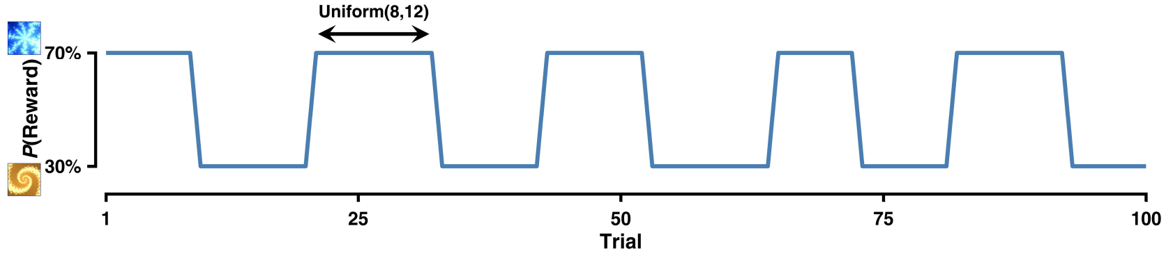
An example reversal learning reward contingency, with reversals every 8-12 trials

In a conventional reversal learning task, participants choose between two stimuli, where initially, one stimulus might have a higher reward probability (say 70%) while the other has a lower probability (30%). However, after a certain number of trials, these probabilities switch or “reverse” - the previously better option becomes the worse option and vice versa. This creates a more challenging learning environment where participants must detect and adapt to these changes. The block length, or the number of trials between each reversal, is also variable; in the example above it is constrained to occur between every 8-12 trials.

Of course, to perform model comparison, we need more than one model! We already have our standard Rescorla-Wagner (RW) model that we’ve used before, so now we will compare it with a variant - the Fictitious (or Counterfactual) RL model.

Recall that the standard RW model updates only the value of the chosen option based on the received reward:

\[V_{t+1}^c = V_t^c + \alpha \cdot PE\]

with the prediction error \(PE\) defined as:

\[PE = R_t - V_t^c\]

where:

\(V_t^c\) is the value of the chosen option,
\(\alpha\) is the learning rate.

The Fictitious RL model extends the basic Rescorla-Wagner by also updating the value of the unchosen option. The key insight is that in binary choice tasks with complementary rewards (like our reversal learning task), not receiving a reward on one option provides information about what might have happened had we chosen the other option.

The model captures this through these equations:

\[V_{t+1}^c = V_t^c + \alpha \cdot PE\] and simultaneously:

\[V_{t+1}^{nc} = V_t^{nc} + \alpha \cdot PE_{nc}\]

where:

\[PE = R_t - V_t^c\] and:

\[PE_{nc} = -R_t - V_t^{nc}\]

The crucial difference are in the second and fourth equations: the model updates the value of the non-chosen option (\(V_t^{nc}\)) using a counterfactual prediction error (\(PE_{nc}\)).

The negative sign before \(R_t\) in \(PE_{nc}\) in the last equation reflects the complementary nature of the rewards - if one option gives a reward, the other option would have given no reward, and vice versa. This counterfactual learning might be particularly useful in reversal learning tasks, as it allows participants to learn about both options on every trial, potentially enabling faster adaptation to reversals.

To better understand the difference between the two models, the graphs below plot the value update calculated by both models with the learning rate (\(η = 0.35\)) and inverse temperature (\(τ = 1.2\)) parameters fixed to be the same for both:

Value and choice predicted by the Fictitious and Rescorla-Wagner (Simple) RL models with fixed learning rates and inverse temperatures

The crucial difference between the models is visible in how the unchosen option’s value changes. In the Simple RL model, the unchosen option’s value remains flat/unchanged until it is chosen again. This creates “plateaus” in the value lines when an option isn’t chosen, for example in the orange line around trials 20-30, where it remains completely flat while option A is being chosen.

Conversely, for the Fictitious RL model, where both options’ values are updated on every trial, no flat plateaus are visible. Subsequently, the value difference between the options for both models, highlights how this is - on average, across all trials - larger for the Fictitious RL model compared to the Simple RL model. As a result, because larger value differences could translate into an easier choice between the two options, the Fictitious RL represents a potential cognitive process that people use.

Now that we have two models, we can compare them directly using PSIS-LOO-CV, and test whether participants actually use this additional information when making decisions in the reversal learning task.

The Stan implementation of the Fictitious RL can be found in _scripts/comparing_models_model2.stan. Comparing this to the Simple RL comparing_models_model1.stan, we can’t see much of a difference. In fact, the only major difference is in the model block.

In the Simple RL, we have a simple update rule that only modifies the value of the chosen option:

pe = reward[s,t] - v[choice[s,t]];
v[choice[s,t]] = v[choice[s,t]] + lr[s] * pe;

This shows that on each trial, the model:

Calculates a prediction error (pe) for the chosen option
Updates only the value of the chosen option using this prediction error

The second model extends this by also updating the unchosen option’s value:

pe = reward[s,t] - v[choice[s,t]];
penc = -reward[s,t] - v[3 - choice[s,t]];

v[choice[s,t]] = v[choice[s,t]] + lr[s] * pe;
v[3 - choice[s,t]] = v[3 - choice[s,t]] + lr[s] * penc;

After declaring a new variable penc for the counterfactual prediction error real penc;:

We use 3 - choice[s,t] to index the unchosen option (since if choice is 1, we want 2, and if choice is 2, we want 1)
We calculate penc using the negative of the reward (-reward[s,t])
We update both the chosen and unchosen options’ values on each trial

Exercise 13

1. Run both models using the R script compare_models_main.R, and examine the LOOIC values for each. Which is best?

Click to reveal the solution

The results should look (roughly⁵) like this:

> LL1 <- extract_log_lik(fit_rl1)
> ( loo1 <- loo(LL1) )
Computed from 4000 by 10 log-likelihood matrix

         Estimate   SE
elpd_loo   -389.4 15.4
p_loo         3.5  0.7
looic       778.7 30.8

> ( loo2 <- loo(LL2) )
Computed from 4000 by 10 log-likelihood matrix

         Estimate   SE
elpd_loo   -281.6 17.5
p_loo         3.8  0.5
looic       563.2 35.1

The lower LOOIC value for the second model (Fictitious RL) (~563 vs ~779) suggests it provides a better fit to the data than the Rescorla-Wagner model.

Posterior predictive checks

We have just compared our two RL models objectively using PSIS-LOO-CV, suggesting that the Fictitious RL model will better predict new, unseen data from our reversal learning task and more accurately captures the underlying latent cognitive processes that generated the observed data. But while quantitative measures like PSIS-LOO-CV help us compare models numerically, posterior predictive checks allow us to visually assess how well our models actually capture patterns in the observed data.

The basic idea of posterior predictive checks is simple: we ask our model to generate simulated data. If our model is good, data simulated from it should look similar to our actual data. Not only does running posterior predictive checks allow us to validate good fitting models, it also can be used to falsify bad fitting ones.

To perform posterior predictive checks, we need to add a section to our Stan models that generates simulated data. We do this in the generated quantities block.

Importantly, because we are using a Bayesian approach, we don’t just simulate from the mean parameter estimates - instead, we simulate new data using every posterior sample of our parameters. This is crucial because it allows us to incorporate our uncertainty about the parameters into our predictions.

From our Stan model, we get posterior samples for all parameters - in our case, 4000 draws from the posterior distribution of each parameter (learning rates, inverse temperatures, etc.). For each of these 4000 parameter sets, we then simulate an entire experiment worth of data using those specific parameters. This is what’s happening in the corresponding generated quantities block:

generated quantities {
  // ... existing code for log likelihood ...

  // Generate predicted choices
  array[nSubjects, nTrials] int y_pred;

  { // local section
    for (s in 1:nSubjects) {
      vector[2] v;
      real pe;
      v = initV;

      for (t in 1:nTrials) {
        // Generate predicted choice from current values
        y_pred[s,t] = categorical_logit_rng(tau[s] * v);

        // Update values using actual reward
        pe = reward[s,t] - v[choice[s,t]];
        v[choice[s,t]] = v[choice[s,t]] + lr[s] * pe;
      }
    }
  }
}

This generates 4000 different simulated datasets. Subsequently, we need to then compare the accuracy of these datasets using R.

Exercise 14

1. Plot the posterior predictive checks for both models (Simple and Fictitious RL) using the R script comparing_models_ppc.R and examine the output.

You should generate the two plots below:

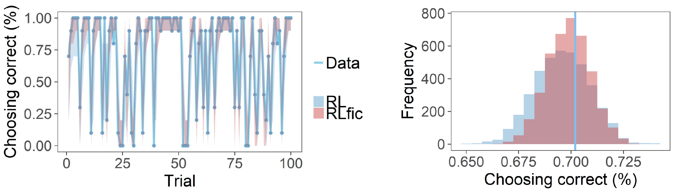
Posterior predictive checks for both models: trial-by-trial choice accuracy (left) and distribution of overall accuracy (right)

For the time course plot on the left, for each trial, we take all 4000 simulated experiments and calculate the proportion of correct choices at that trial across all subjects.

For the distribution plot on the right, for each of the 4000 simulated experiments, we calculate the overall proportion of correct choices across all trials and subjects. The histograms show the distribution of these 4000 overall proportions, whilst the vertical line shows the actual overall proportion from the real data.

Again, you can see that the straight blue line is closer to the peak for the Fictitious RL compared to the simple RL, demonstrating that this model better captures the true choice behaviour patterns in the data.

Footnotes

Pitt, M. A., & Myung, I. J. (2002). When a good fit can be bad. Trends in cognitive sciences, 6(10), 421-425.↩︎
Vehtari, A., Gelman, A., & Gabry, J. (2017). Practical Bayesian model evaluation using leave-one-out cross-validation and WAIC. Statistics and Computing, 27, 1413-1432.↩︎
Vehtari, A., Gabry, J., Magnusson, M., Yao, Y., Bürkner, P., Paananen, T., & Gelman, A. (2024). loo: Efficient leave-one-out cross-validation and WAIC for Bayesian models (Version 2.8.0) [R package]. Retrieved from https://mc-stan.org/loo/↩︎
Zhang, L., & Gläscher, J. (2020). A brain network supporting social influences in human decision-making. Science advances, 6(34), eabb4159.↩︎
Even though the Stan model code in R uses the same seed, differences in hardware across computers will produce slightly different end results.↩︎